Plot static scatterplot matrix. Optionally, superimpose differentially expressed genes (DEGs) onto scatterplot matrix.
plotSM(
  data = data,
  dataMetrics = NULL,
  dataSE = NULL,
  geneList = NULL,
  threshVar = "FDR",
  threshVal = 0.05,
  option = c("allPoints", "foldChange", "orthogonal", "hexagon"),
  xbins = 10,
  threshFC = 3,
  threshOrth = 3,
  pointSize = 0.5,
  pointColor = "orange",
  outDir = tempdir(),
  saveFile = TRUE
)
Arguments
| data | DATA FRAME | Read counts |
|---|---|
| dataMetrics | LIST | Differential expression metrics; default NULL |
| dataSE | SUMMARIZEDEXPERIMENT | Summarized experiment format that can be used in lieu of data and dataMetrics; default NULL |
| geneList | CHARACTER ARRAY | List of gene IDs to be drawn onto the scatterplot matrix of all data. Use this parameter if you have predetermined genes to be drawn. Otherwise, use dataMetrics, threshVar, and threshVal to create genes to be drawn onto the scatterplot matrix; default NULL; used in "hexagon" and "allPoints" |
| threshVar | CHARACTER STRING | Name of column in dataMetrics object that is used to threshold significance; default "FDR"; used in all options |
| threshVal | INTEGER | Maximum value to threshold significance from threshVar object; default 0.05; used in all options |
| option | CHARACTER STRING ["foldChange" | "orthogonal" | "hexagon" | "allPoints"] | The type of plot; default "allPoints" |
| xbins | INTEGER | Number of bins partitioning the range of the plot; default 10; used in option "hexagon" |
| threshFC | INTEGER | Threshold of fold change; default 3; used in option "foldChange" |
| threshOrth | INTEGER | Threshold of orthogonal distance; default 3; used in option "orthogonal" |
| pointSize | INTEGER | Size of plotted points; default 0.5; used for DEGs in "hexagon" and "allPoints" and used for all points in "foldChange" and "orthogonal" |
| pointColor | CHARACTER STRING | Color of overlaid points on scatterplot matrix; default "orange"; used for DEGs in "hexagon" and "allPoints" and used for all points in "foldChange" and "orthogonal" |
| outDir | CHARACTER STRING | Output directory to save all plots; default tempdir(); used in all options |
| saveFile | BOOLEAN [TRUE | FALSE] | Save file to outDir; default TRUE; used in all options |
Value
List of n elements of scatterplot matrices, where n is the number of treatment pair combinations in the data object. The subset of genes that are superimposed are determined through the dataMetrics or geneList parameter. If the saveFile parameter has a value of TRUE, then each of these scatterplot matrices is saved to the location specified in the outDir parameter as a JPG file.
Details
There are seven options:
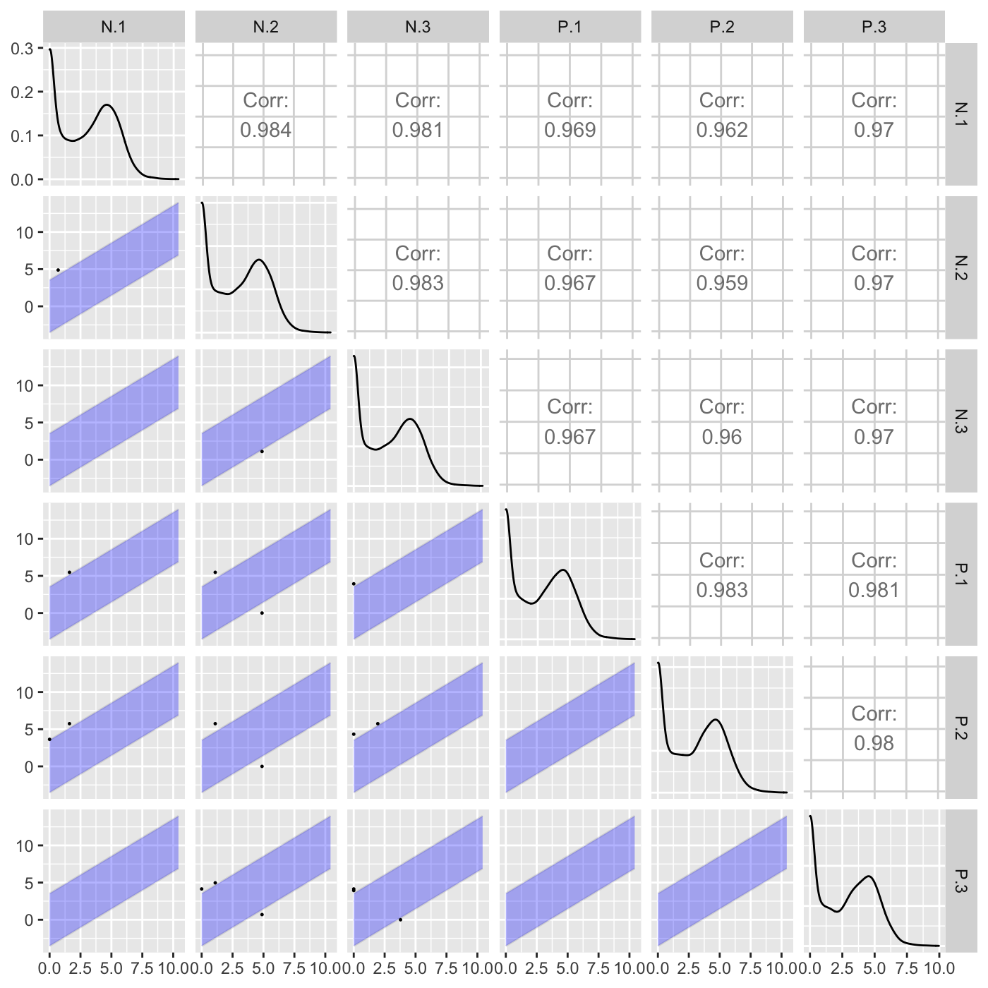
"foldChange": Plots DEGs onto scatterplot matrix of fold changes
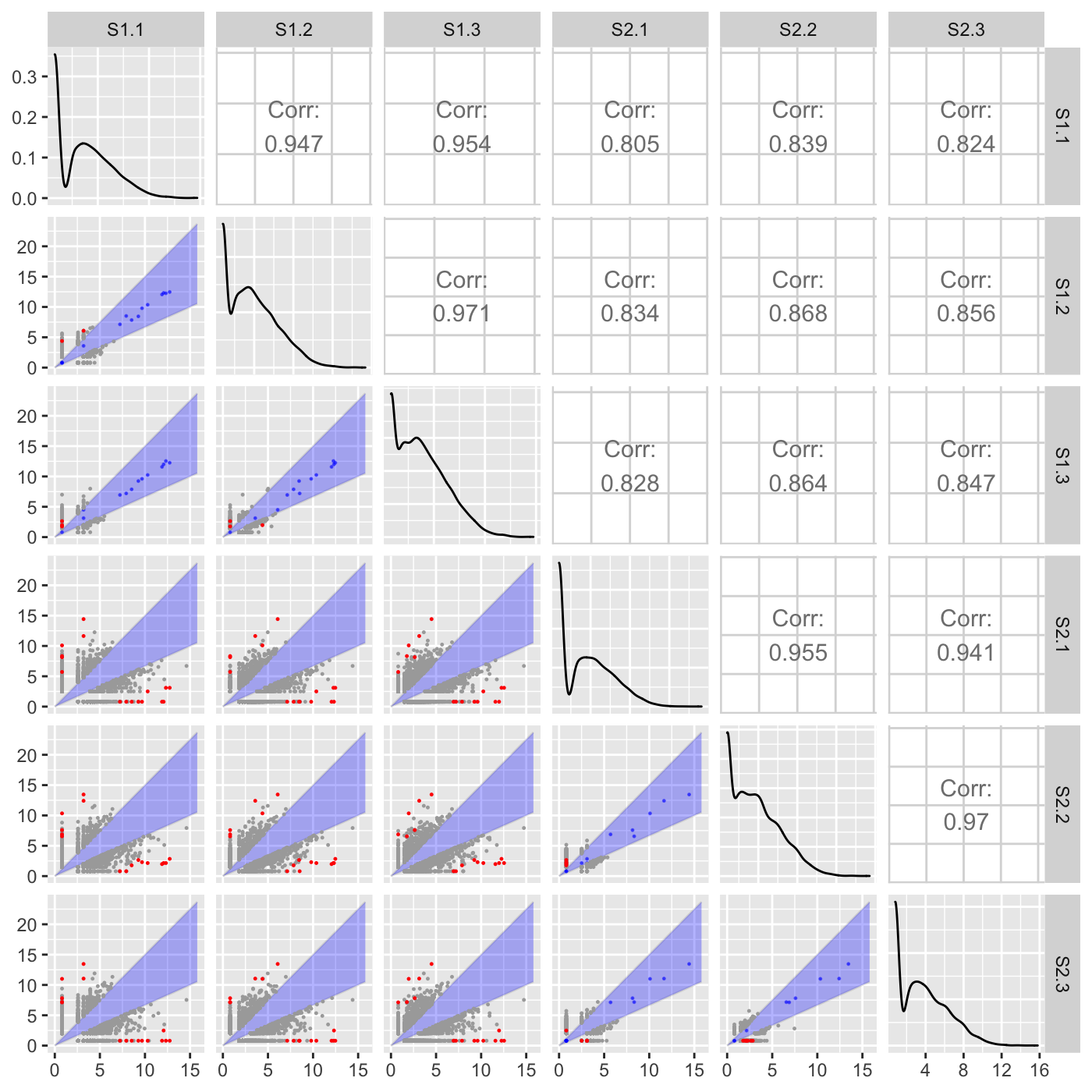
"orthogonal": Plots DEGs onto scatterplot matrix of orthogonal distance
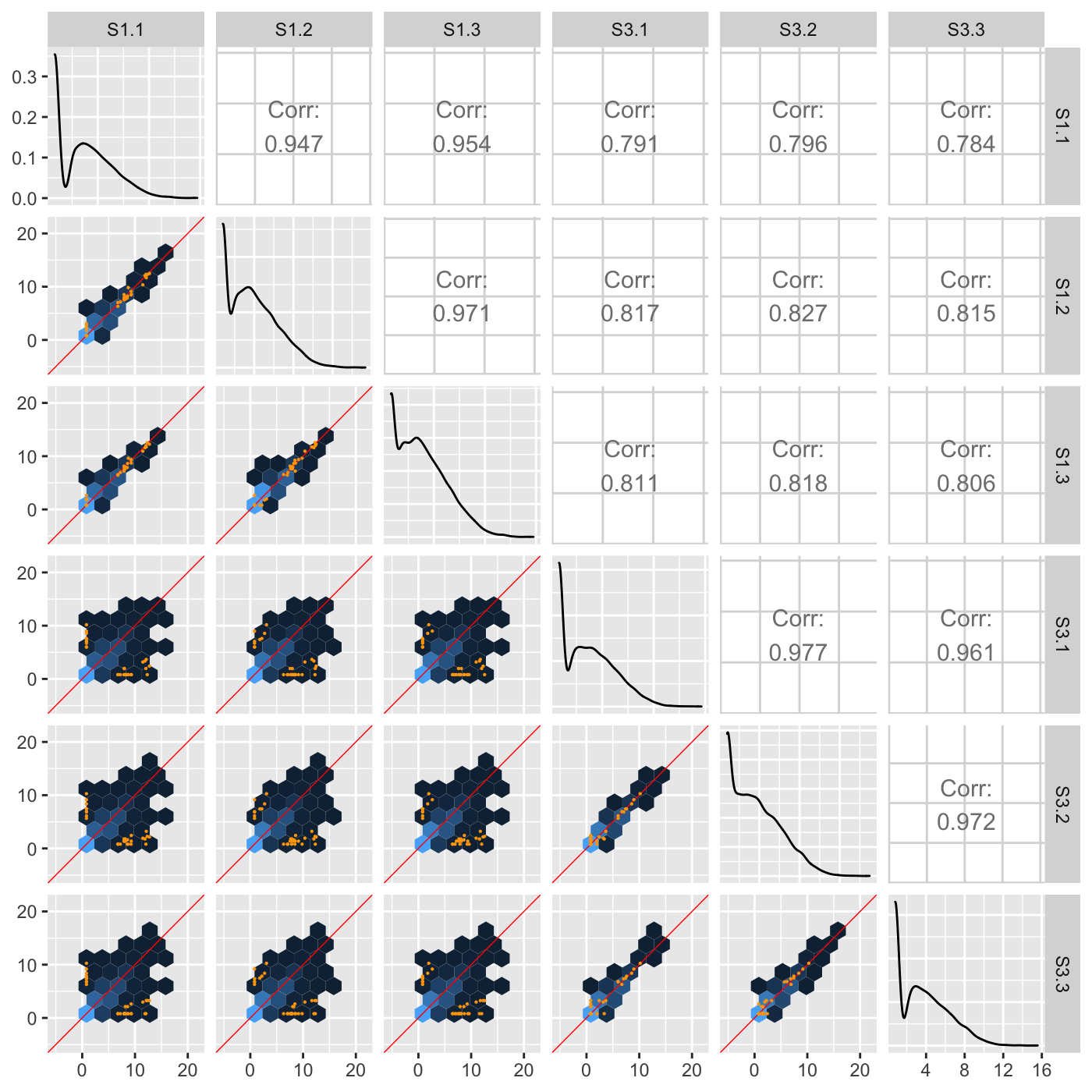
"hexagon": Plot DEGs onto scatterplot matrix of hexagon binning
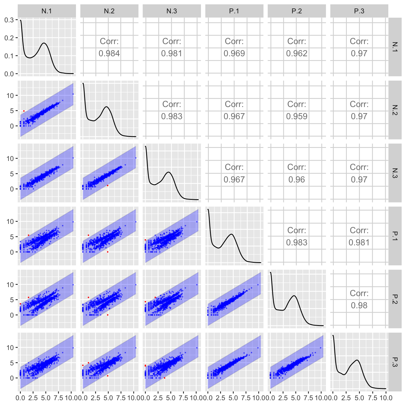
"allPoints": Plot DEGs onto scatterplot matrix of all data points
Examples
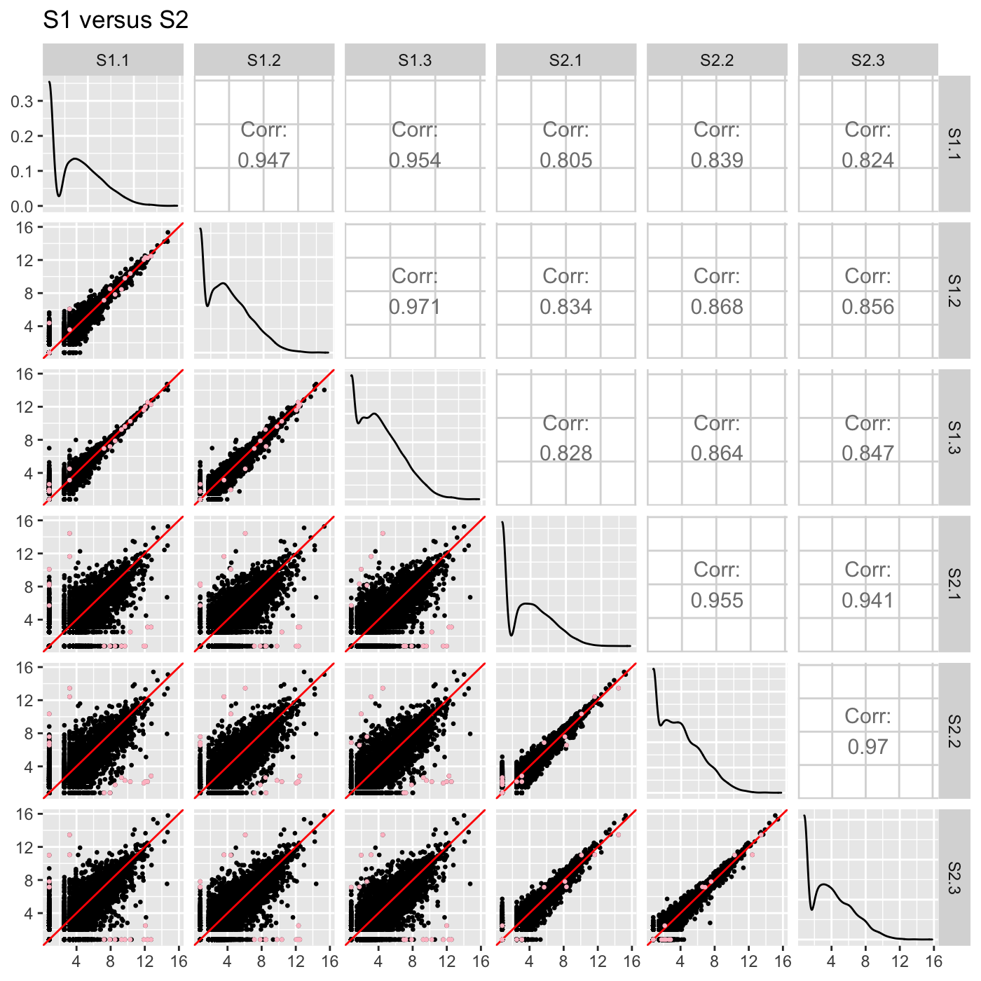
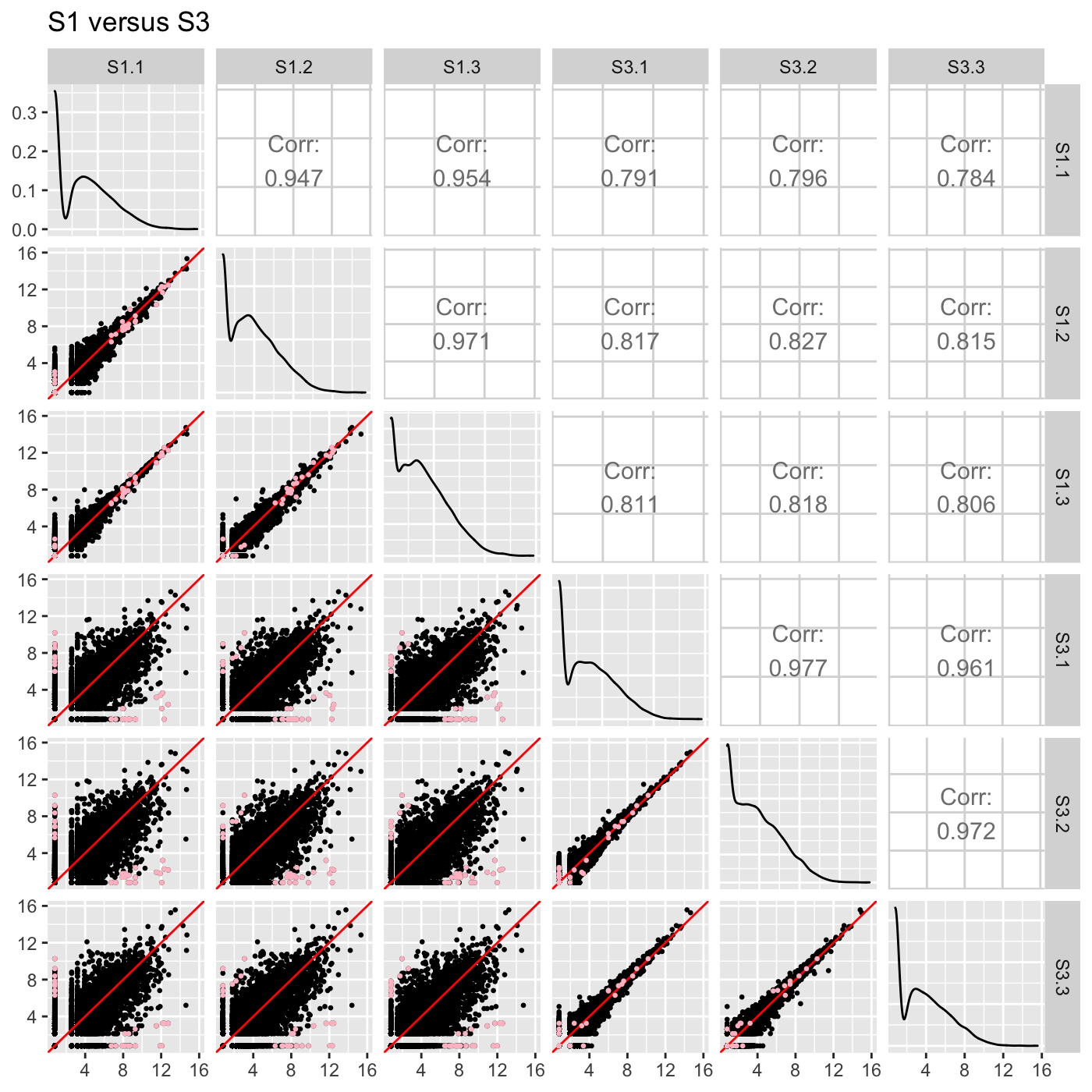
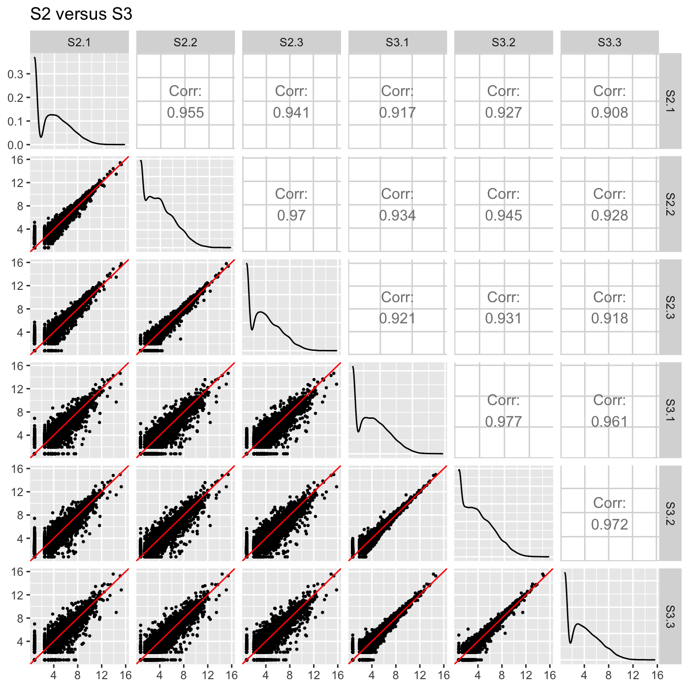
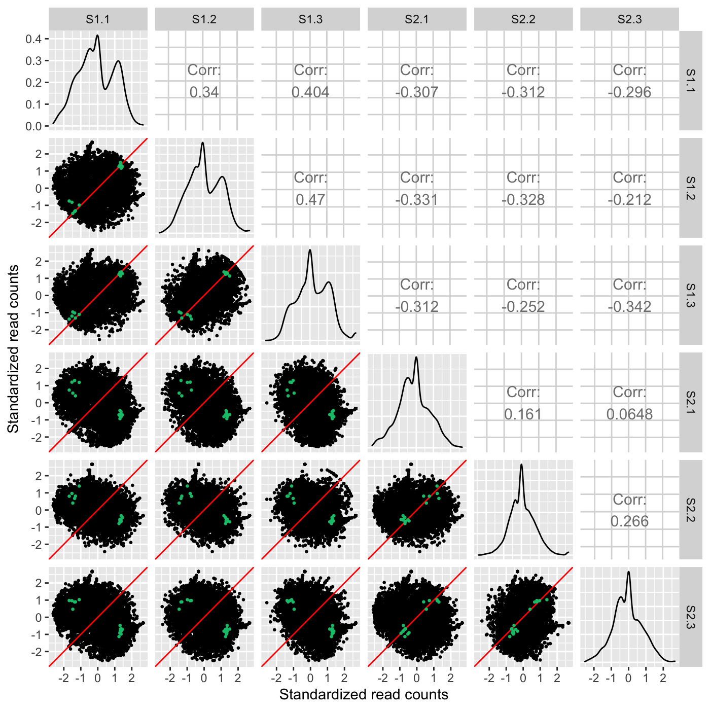
# The first set of six examples use data and dataMetrics # objects as input. The last set of six examples create the same plots now # using the SummarizedExperiment (i.e. dataSE) object input. # Read in data and metrics (need for first set of six examples) data(soybean_cn_sub) data(soybean_cn_sub_metrics) data(soybean_ir_sub) data(soybean_ir_sub_metrics) # Create standardized version of data (need for first set of six examples) library(matrixStats) library(ggplot2) soybean_cn_sub_st <- as.data.frame(t(apply(as.matrix(soybean_cn_sub[,-1]), 1, scale))) soybean_cn_sub_st$ID <- as.character(soybean_cn_sub$ID) soybean_cn_sub_st <- soybean_cn_sub_st[,c(length(soybean_cn_sub_st), 1:length(soybean_cn_sub_st)-1)] colnames(soybean_cn_sub_st) <- colnames(soybean_cn_sub) nID <- which(is.nan(soybean_cn_sub_st[,2])) soybean_cn_sub_st[nID,2:length(soybean_cn_sub_st)] <- 0 # Example 1: Plot scatterplot matrix of points. Saves three plots to outDir # because saveFile equals TRUE by default. if (FALSE) { plotSM(soybean_cn_sub, soybean_cn_sub_metrics) } # Example 2: Plot scatterplot matrix of points. Return list of plots so user # can tailor them (such as add title) and does not save to outDir because # saveFile equals FALSE. ret <- plotSM(soybean_cn_sub, soybean_cn_sub_metrics, pointColor = "pink", saveFile = FALSE) # Determine names of plots in returned list names(ret)#> [1] "S1_S2" "S1_S3" "S2_S3"#> Warning: Using `as.character()` on a quosure is deprecated as of rlang 0.3.0. #> Please use `as_label()` or `as_name()` instead. #> This warning is displayed once per session.# Example 3: Plot standardized data as scatterplot matrix of points. ret <- plotSM(soybean_cn_sub_st, soybean_cn_sub_metrics, pointColor = "#00C379", saveFile = FALSE) ret[[1]] + xlab("Standardized read counts") + ylab("Standardized read counts")# Example 4: Plot scatterplot matrix of hexagons. ret <- plotSM(soybean_cn_sub, soybean_cn_sub_metrics, option = "hexagon", xbins = 5, pointSize = 0.1, saveFile = FALSE) ret[[2]]# Example 5: Plot scatterplot matrix of orthogonal distance on the logged # data, first without considering the metrics dataset and then considering # it. soybean_ir_sub[,-1] <- log(soybean_ir_sub[,-1] + 1) ret <- plotSM(soybean_ir_sub, option = "orthogonal", threshOrth = 2.5, pointSize = 0.2, saveFile = FALSE) ret[[1]]ret <- plotSM(soybean_ir_sub, soybean_ir_sub_metrics, option = "orthogonal", threshOrth = 2.5, pointSize = 0.2, saveFile = FALSE) ret[[1]]# Example 6: Plot scatterplot matrix of fold change. ret <- plotSM(soybean_cn_sub, soybean_cn_sub_metrics, option = "foldChange", threshFC = 0.5, pointSize = 0.2, saveFile = FALSE) ret[[1]]# Below are the same six examples, only now using the # SummarizedExperiment (i.e. dataSE) object as input. # Read in data and metrics (need for first set of six examples) data(se_soybean_cn_sub) data(se_soybean_ir_sub) # Create standardized version of data (need for first set of six examples) library(matrixStats) library(ggplot2) library(SummarizedExperiment) se_soybean_cn_sub_st = se_soybean_cn_sub assay(se_soybean_cn_sub_st, withDimnames=FALSE) <-as.data.frame(t( apply(as.matrix(as.data.frame(assay(se_soybean_cn_sub))), 1, scale))) nID <- which(is.nan(as.data.frame(assay(se_soybean_cn_sub_st))[,1])) assay(se_soybean_cn_sub_st, withDimnames=FALSE)[nID,] <- 0 # Example 1: Plot scatterplot matrix of points. Saves three plots to outDir # because saveFile equals TRUE by default. if (FALSE) { plotSM(dataSE = se_soybean_cn_sub) } # Example 2: Plot scatterplot matrix of points. Return list of plots so user # can tailor them (such as add title) and does not save to outDir because # saveFile equals FALSE. if (FALSE) { ret <- plotSM(dataSE = se_soybean_cn_sub, pointColor = "pink", saveFile = FALSE) # Determine names of plots in returned list names(ret) ret[["S1_S2"]] + ggtitle("S1 versus S2") ret[["S1_S3"]] + ggtitle("S1 versus S3") ret[["S2_S3"]] + ggtitle("S2 versus S3") } # Example 3: Plot standardized data as scatterplot matrix of points. if (FALSE) { ret <- plotSM(dataSE = se_soybean_cn_sub_st, pointColor = "#00C379", saveFile = FALSE) ret[[1]] + xlab("Standardized read counts") + ylab("Standardized read counts") } # Example 4: Plot scatterplot matrix of hexagons. if (FALSE) { ret <- plotSM(dataSE = se_soybean_cn_sub, option = "hexagon", xbins = 5, pointSize = 0.1, saveFile = FALSE) ret[[2]] } # Example 5: Plot scatterplot matrix of orthogonal distance on the logged # data, first without considering the metrics dataset and then considering # it. if (FALSE) { assay(se_soybean_ir_sub) <- log(as.data.frame(assay(se_soybean_ir_sub))+1) ret <- plotSM(dataSE = se_soybean_ir_sub, option = "orthogonal", threshOrth = 2.5, pointSize = 0.2, saveFile = FALSE) ret[[1]] } # Example 6: Plot scatterplot matrix of fold change. if (FALSE) { ret <- plotSM(dataSE = se_soybean_cn_sub, option = "foldChange", threshFC = 0.5, pointSize = 0.2, saveFile = FALSE) ret[[1]] }